
Campaign Budget Optimizer
Table of Contents
- Project Overview
- Business Problem and Objectives
- Data Sources and Preparation
- Exploratory Data Analysis
- Predictive Modeling and Model Selection
- Budget Optimization
- Interactive Application
- Results and Business Insights
- Limitations and Future Improvements
- References and Full Case Study
Public demonstration. All campaign names, input data, fitted parameters, budgets, and results in this page are synthetic and illustrative. They are not company data or validated production results. The original implementation, operational configuration, and proprietary data are not published.
Project Overview
How should a marketing team distribute a fixed advertising budget across campaigns with different acquisition costs and diminishing returns?
I developed a decision-support workflow combining campaign response modeling, out-of-sample model evaluation, and constrained numerical optimization. Its purpose is to compare potential budget allocations and estimate the associated lead volumes and blended cost per lead (CPL).
The project follows a practical sequence: historical spend and leads → model estimation → validation → budget constraints → optimized allocation → interactive scenario comparison.
Business Problem and Objectives
Allocating spend in proportion to historical CPL can be misleading: campaign performance may change as investment increases. A campaign with an attractive average CPL is not necessarily the best destination for the next incremental euro.
The optimization objective is to maximize expected leads for a chosen budget, while keeping each campaign’s spend within operationally feasible limits. The interface also reports the implied blended CPL and allows manual scenario adjustments.
Data Sources and Preparation
The modeling dataset is organized at daily × campaign level. The public example uses anonymized campaign labels and fabricated observations.
| Field | Description |
|---|---|
date | Observation date |
campaign | Anonymous campaign identifier (A, B, C, …) |
spend | Daily advertising spend, in synthetic currency units |
leads | Daily lead count |
The preparation workflow checks missing dates, duplicates, zero-spend observations, inconsistent attribution, and extreme values. It then creates a consistent training dataset and preserves chronological ordering for validation.
Important: The model captures associations in observed spend and leads. Without experimental variation or additional controls, its response curves should not be interpreted as causal incremental lift.
Exploratory Data Analysis
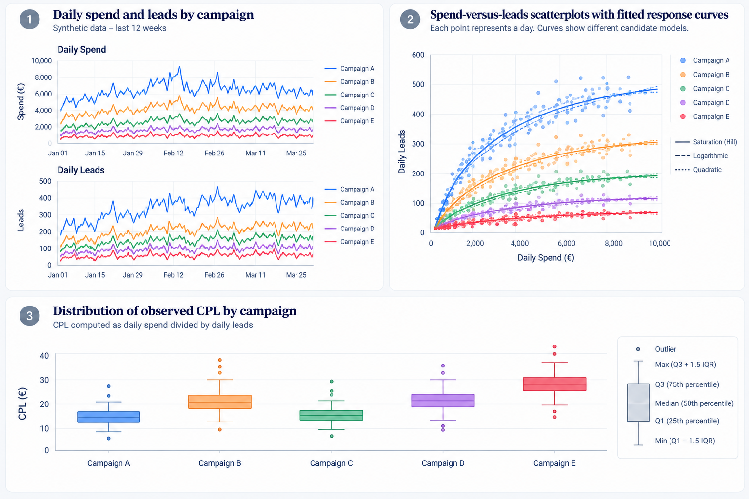
Before fitting models, I inspect the daily spend distribution, lead volumes, CPL, and the relationship between spend and leads for each campaign. The central question is whether a linear response is adequate or whether diminishing returns are visible.
Predictive Modeling and Model Selection
Several functional forms are compared rather than assuming one universal response curve:
| Model | Illustrative form | Interpretation |
|---|---|---|
| Linear | \(f(x)=a+bx\) | Constant marginal response |
| Logarithmic | \(f(x)=a+b\log(1+x)\) | Gradual diminishing returns |
| Quadratic | \(f(x)=a+bx+cx^2\) | Flexible curvature within observed range |
| Saturation | \(f(x)=Lx/(K+x)\) | Response approaches a ceiling |
| Hill | \(f(x)=Lx^h/(K^h+x^h)\) | Flexible S-shaped or saturating response |
| Spend-trend baseline | Trend-based benchmark | Comparison against simpler forecasting behavior |
Here, \(x\) denotes daily spend and \(f(x)\) the predicted daily leads. Model forms are illustrative; exact fitting choices and constraints are implementation-dependent.
Validation
Models are assessed using R², MAE, and RMSE, complemented by chronological out-of-sample MAE, RMSE, normalized RMSE, and prediction bias. A high in-sample R² is not sufficient: the preferred model must also generalize to unseen periods and behave plausibly at the proposed spend levels.
A robust evaluation also checks whether a response curve yields unrealistic negative predictions or implausible increases outside the observed spend range. Where necessary, predictions are bounded or the feasible spend domain is restricted.
Budget Optimization
Let \(x_i\) be the daily budget allocated to campaign \(i\), and \(f_i(x_i)\) its predicted daily leads. The allocation problem is:
\[\max_{x_1,\ldots,x_n}\;\sum_{i=1}^{n} f_i(x_i)\]subject to:
\[\sum_{i=1}^{n}x_i=B,\qquad l_i\leq x_i\leq u_i.\]Here \(B\) is the available daily budget, and \(l_i,u_i\) are campaign-specific feasible limits. A practical approach derives those limits from historical spend ranges, with a configurable upper buffer. Before optimization, the system checks feasibility: \(\sum_i l_i\leq B\leq\sum_i u_i\).
The resulting estimated blended CPL is:
\[\widehat{\mathrm{CPL}}=\frac{B}{\sum_i f_i(x_i)}.\]For nonlinear and potentially non-concave response functions, solver output should be checked using multiple starting points or comparable robustness checks; a numerical solution is not automatically a guaranteed global optimum.
Interactive Application
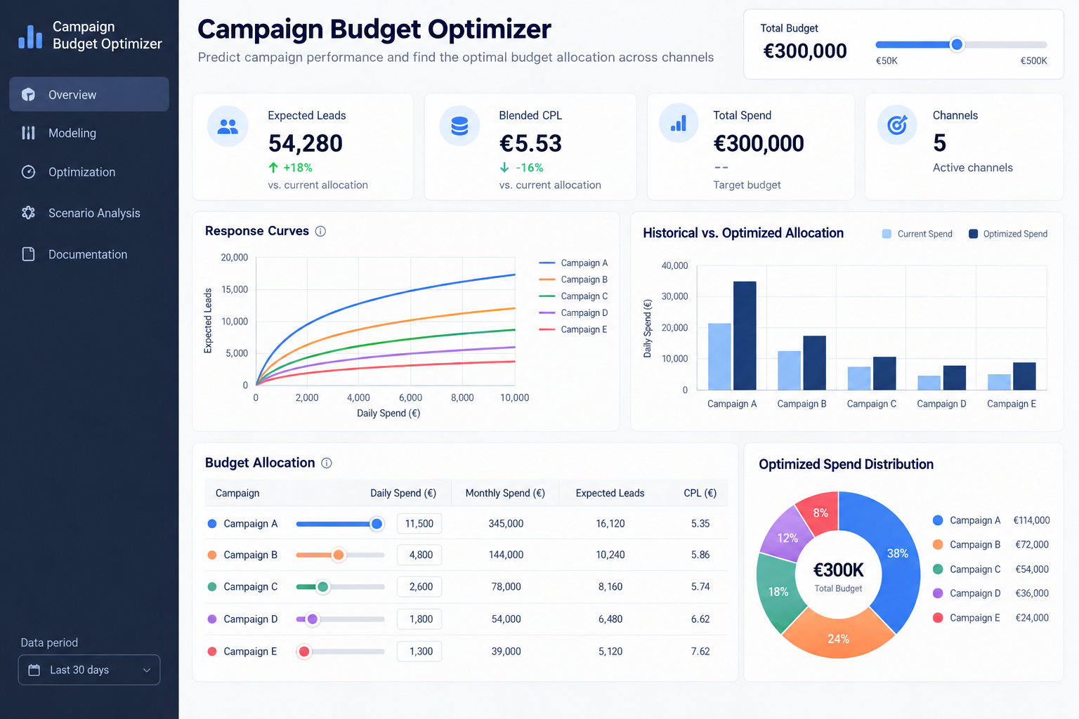
The project is designed around an interactive Streamlit interface for scenario planning. A user can select a total budget, inspect campaign-level allocations, and manually adjust campaign spend through sliders.
The application reports predicted leads, estimated blended CPL, and the difference between a user-defined scenario and a model-suggested allocation.
Results and Business Insights
To illustrate the output, consider a fully fabricated three-campaign scenario:
| Campaign | Baseline daily spend | Example optimized spend |
|---|---|---|
| Campaign A | 300 | 250 |
| Campaign B | 400 | 470 |
| Campaign C | 300 | 280 |
| Total | 1,000 | 1,000 |
The table demonstrates reallocation at a constant total budget. It is not an empirical performance claim: lead gains and CPL improvements must be computed from fitted synthetic curves before displaying them as numerical results.
The main decision-making insight is that marginal expected performance matters more than historical average CPL. Scenario planning makes the trade-offs explicit and helps identify campaigns where additional spend may be less productive.
Limitations and Future Improvements
- Observational bias: spend may react to demand, seasonality, or platform bidding decisions, so fitted relationships are not necessarily causal.
- Short history: limited windows can produce unstable nonlinear parameters and unreliable extrapolation.
- Attribution: platform-reported conversions may differ in definitions, windows, or completeness.
- Uncertainty: point estimates do not convey the range of possible lead outcomes.
- Constraints: historical spend bounds are pragmatic, not proof of operational feasibility.
Future work could include longer historical windows, seasonality controls, uncertainty intervals, more systematic backtesting, and experimental calibration of marginal returns.
References and Full Case Study
Further reading
Request the technical case study
The public page intentionally omits proprietary source code, production data, fitted business parameters, and internal architecture. A deeper walkthrough of modeling choices, validation, optimization, and interface design may be discussed upon request, subject to confidentiality and sharing permissions.
Contact: Request a Technical Case Study
This page documents the approach using synthetic examples; it does not expose or reproduce an employer’s confidential implementation.